
GAN Evaluation : the Frechet Inception Distance and Inception Score metrics
In this notebook, two PyTorch-Ignite’s metrics to evaluate Generative Adversarial Networks (or GAN in short) are introduced :
- Frechet Inception Distance, details can be found in
Heusel et al. 2002 - Inception Score, details can be found in
Barratt et al. 2018
See here for more details about the implementation of the metrics in PyTorch-Ignite.
Most of the code here is from
DCGAN example in
pytorch/examples. In addition to the original tutorial, this notebook will use in-built GAN based metric in ignite.metrics to evaluate Frechet Inception Distnace and Inception Score and showcase other metric based features in ignite.
Required Dependencies
Pytorch, Torchvision and Pytorch-Ignite are the required dependencies. They will be installed/imported here.
!pip install pytorch-ignite
Collecting pytorch-ignite
Downloading pytorch_ignite-0.4.6-py3-none-any.whl (232 kB)
[K |████████████████████████████████| 232 kB 8.1 MB/s eta 0:00:01
[?25hRequirement already satisfied: torch<2,>=1.3 in /usr/local/lib/python3.7/dist-packages (from pytorch-ignite) (1.9.0+cu102)
Requirement already satisfied: typing-extensions in /usr/local/lib/python3.7/dist-packages (from torch<2,>=1.3->pytorch-ignite) (3.7.4.3)
Installing collected packages: pytorch-ignite
Successfully installed pytorch-ignite-0.4.6
import torch
import torchvision
import ignite

print(*map(lambda m: ": ".join((m.__name__, m.__version__)), (torch, torchvision, ignite)), sep="\n")
torch: 1.9.0+cu102
torchvision: 0.10.0+cu102
ignite: 0.4.6
Import Libraries
Note: torchsummary is an optional dependency here.
import os
import logging
import matplotlib.pyplot as plt

import numpy as np

from torchsummary import summary

import torch
import torch.nn as nn
import torch.optim as optim

import torchvision.transforms as transforms
import torchvision.utils as vutils

from ignite.engine import Engine, Events
import ignite.distributed as idist
Reproductibility and logging details
ignite.utils.manual_seed(999)
Optionally, the logging level logging.WARNING is used in internal ignite submodules in order to avoid internal messages.
ignite.utils.setup_logger(name="ignite.distributed.auto.auto_dataloader", level=logging.WARNING)
ignite.utils.setup_logger(name="ignite.distributed.launcher.Parallel", level=logging.WARNING)
<Logger ignite.distributed.launcher.Parallel (WARNING)>
Processing Data
The
Large-scale CelebFaces Attributes (CelebA) Dataset is used in this tutorial. The torchvision library provides a
dataset class, However this implementation suffers from issues related to the download limitations of gdrive. Here, we define a custom CelebA
Dataset.
from torchvision.datasets import ImageFolder
!gdown --id 1O8LE-FpN79Diu6aCvppH5HwlcR5I--PX
!mkdir data
!unzip -qq img_align_celeba.zip -d data
Downloading...
From: https://drive.google.com/uc?id=1O8LE-FpN79Diu6aCvppH5HwlcR5I--PX
To: /content/img_align_celeba.zip
1.44GB [00:13, 107MB/s]
Dataset and transformation
The image size considered in this tutorial is 64. Note that increase this size implies to modify the GAN models.
image_size = 64

data_transform = transforms.Compose(
    [
        transforms.Resize(image_size),
        transforms.CenterCrop(image_size),
        transforms.ToTensor(),
        transforms.Normalize((0.5, 0.5, 0.5), (0.5, 0.5, 0.5)),
    ]
)

train_dataset = ImageFolder(root="./data", transform=data_transform)
test_dataset = torch.utils.data.Subset(train_dataset, torch.arange(3000))
DataLoading
We wish to configure the dataloader to work in a disbtributed environment. Distributed Dataloading is support by Ignite as part of DDP support. This requires specific adjustments to the sequential case.
To handle this, idist provides an helper
auto_dataloader which automatically distributes the data over the processes.
Note: Distributed dataloading is described in Distributed Data Parallel (DDP) tutorial if you wish to learn more.
batch_size = 128

train_dataloader = idist.auto_dataloader(
    train_dataset,
    batch_size=batch_size,
    num_workers=2,
    shuffle=True,
    drop_last=True,
)

test_dataloader = idist.auto_dataloader(
    test_dataset,
    batch_size=batch_size,
    num_workers=2,
    shuffle=False,
    drop_last=True,
)
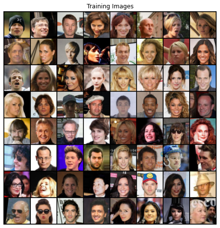
Let’s explore the data.
real_batch = next(iter(train_dataloader))

plt.figure(figsize=(8,8))
plt.axis("off")
plt.title("Training Images")
plt.imshow(np.transpose(vutils.make_grid(real_batch[0][:64], padding=2, normalize=True).cpu(),(1,2,0)))
plt.show()
Models for GAN
Generator
The latent space dimension of input vectors for the generator is a key parameter of GAN.
latent_dim = 100
class Generator3x64x64(nn.Module):
    def __init__(self, latent_dim):
        super(Generator3x64x64, self).__init__()
        self.model = nn.Sequential(
            nn.ConvTranspose2d(latent_dim, 512, 4, 1, 0, bias=False),
            nn.BatchNorm2d(512),
            nn.ReLU(True),
            # state size. 512 x 4 x 4
            nn.ConvTranspose2d(512, 256, 4, 2, 1, bias=False),
            nn.BatchNorm2d(256),
            nn.ReLU(True),
            # state size. 256 x 8 x 8
            nn.ConvTranspose2d(256, 128, 4, 2, 1, bias=False),
            nn.BatchNorm2d(128),
            nn.ReLU(True),
            # state size. 128 x 16 x 16
            nn.ConvTranspose2d(128, 64, 4, 2, 1, bias=False),
            nn.BatchNorm2d(64),
            nn.ReLU(True),
            # state size. 64 x 32 x 32
            nn.ConvTranspose2d(64, 3, 4, 2, 1, bias=False),
            nn.Tanh()
            # final state size. 3 x 64 x 64
        )

    def forward(self, x):
        x = self.model(x)
        return x
As for dataloading, distributed models requires some specifics that idist adresses providing the
auto_model helper.
netG = idist.auto_model(Generator3x64x64(latent_dim))
Note that the model is automatically moved to the best device detected by idist.
idist.device()
device(type='cuda')
summary(netG, (latent_dim, 1, 1))
----------------------------------------------------------------
        Layer (type)               Output Shape         Param #
================================================================
   ConvTranspose2d-1            [-1, 512, 4, 4]         819,200
       BatchNorm2d-2            [-1, 512, 4, 4]           1,024
              ReLU-3            [-1, 512, 4, 4]               0
   ConvTranspose2d-4            [-1, 256, 8, 8]       2,097,152
       BatchNorm2d-5            [-1, 256, 8, 8]             512
              ReLU-6            [-1, 256, 8, 8]               0
   ConvTranspose2d-7          [-1, 128, 16, 16]         524,288
       BatchNorm2d-8          [-1, 128, 16, 16]             256
              ReLU-9          [-1, 128, 16, 16]               0
  ConvTranspose2d-10           [-1, 64, 32, 32]         131,072
      BatchNorm2d-11           [-1, 64, 32, 32]             128
             ReLU-12           [-1, 64, 32, 32]               0
  ConvTranspose2d-13            [-1, 3, 64, 64]           3,072
             Tanh-14            [-1, 3, 64, 64]               0
================================================================
Total params: 3,576,704
Trainable params: 3,576,704
Non-trainable params: 0
----------------------------------------------------------------
Input size (MB): 0.00
Forward/backward pass size (MB): 3.00
Params size (MB): 13.64
Estimated Total Size (MB): 16.64
----------------------------------------------------------------
Discriminator
class Discriminator3x64x64(nn.Module):
    def __init__(self):
        super(Discriminator3x64x64, self).__init__()
        self.model = nn.Sequential(
            # input is 3 x 64 x 64
            nn.Conv2d(3, 64, 4, 2, 1, bias=False),
            nn.LeakyReLU(0.2, inplace=True),
            # state size. 64 x 32 x 32
            nn.Conv2d(64, 128, 4, 2, 1, bias=False),
            nn.BatchNorm2d(128),
            nn.LeakyReLU(0.2, inplace=True),
            # state size. 128 x 16 x 16
            nn.Conv2d(128, 256, 4, 2, 1, bias=False),
            nn.BatchNorm2d(256),
            nn.LeakyReLU(0.2, inplace=True),
            # state size. 256 x 8 x 8
            nn.Conv2d(256, 512, 4, 2, 1, bias=False),
            nn.BatchNorm2d(512),
            nn.LeakyReLU(0.2, inplace=True),
            # state size. 512 x 4 x 4
            nn.Conv2d(512, 1, 4, 1, 0, bias=False),
            nn.Sigmoid()
        )

    def forward(self, x):
        x = self.model(x)
        return x
netD = idist.auto_model(Discriminator3x64x64())
summary(netD, (3, 64, 64))
----------------------------------------------------------------
        Layer (type)               Output Shape         Param #
================================================================
            Conv2d-1           [-1, 64, 32, 32]           3,072
         LeakyReLU-2           [-1, 64, 32, 32]               0
            Conv2d-3          [-1, 128, 16, 16]         131,072
       BatchNorm2d-4          [-1, 128, 16, 16]             256
         LeakyReLU-5          [-1, 128, 16, 16]               0
            Conv2d-6            [-1, 256, 8, 8]         524,288
       BatchNorm2d-7            [-1, 256, 8, 8]             512
         LeakyReLU-8            [-1, 256, 8, 8]               0
            Conv2d-9            [-1, 512, 4, 4]       2,097,152
      BatchNorm2d-10            [-1, 512, 4, 4]           1,024
        LeakyReLU-11            [-1, 512, 4, 4]               0
           Conv2d-12              [-1, 1, 1, 1]           8,192
          Sigmoid-13              [-1, 1, 1, 1]               0
================================================================
Total params: 2,765,568
Trainable params: 2,765,568
Non-trainable params: 0
----------------------------------------------------------------
Input size (MB): 0.05
Forward/backward pass size (MB): 2.31
Params size (MB): 10.55
Estimated Total Size (MB): 12.91
----------------------------------------------------------------
Optimizers
The Binary Cross Entropy Loss is used in this tutorial.
criterion = nn.BCELoss()
A batch of 64 fixed samples will be used for generating images from throughout the training. This will allow a qualitative evaluation throughout the training progress.
fixed_noise = torch.randn(64, latent_dim, 1, 1, device=idist.device())
Finally, two separate optimizers are set up, one for the generator, and one for the discriminator. Yet, another helper method
auto_optim provided by idist will help to adapt optimizer for distributed configurations.
optimizerD = idist.auto_optim(
    optim.Adam(netD.parameters(), lr=0.0002, betas=(0.5, 0.999))
)

optimizerG = idist.auto_optim(
    optim.Adam(netG.parameters(), lr=0.0002, betas=(0.5, 0.999))
)
Ignite Training Concepts
Training in Ignite is based on three core components, namely, Engine, Events and Handlers. Let’s briefly discuss each of them.
-
Engine - The Engine can be considered somewhat similar to a training loop. It takes a
train_stepas an argument and runs it over each batch of the dataset, triggering events as it goes. -
Events - Events are emitted by the Engine when it reaches a specific point in the run/training.
-
Handlers - Functions that can be triggered when a certain Event is emitted by the Engine. Ignite has a long list of pre defined Handlers such as checkpoint, early stopping, logging and built-in metrics, see ignite-handlers.
Training Step Function
A training step function will be run batch wise over the entire dataset by the engine. It contains the basic training steps, namely, running the model, propagating the loss backward and taking an optimizer step. We run the discriminator model on both real images and fake images generated by the Generator model. The function returns Generator and Discriminator Losses and the output generated by Generator and Discriminator.
real_label = 1
fake_label = 0


def training_step(engine, data):
    # Set the models for training
    netG.train()
    netD.train()

    ############################
    # (1) Update D network: maximize log(D(x)) + log(1 - D(G(z)))
    ###########################
    ## Train with all-real batch
    netD.zero_grad()
    # Format batch
    real = data[0].to(idist.device())
    b_size = real.size(0)
    label = torch.full((b_size,), real_label, dtype=torch.float, device=idist.device())
    # Forward pass real batch through D
    output1 = netD(real).view(-1)
    # Calculate loss on all-real batch
    errD_real = criterion(output1, label)
    # Calculate gradients for D in backward pass
    errD_real.backward()

    ## Train with all-fake batch
    # Generate batch of latent vectors
    noise = torch.randn(b_size, latent_dim, 1, 1, device=idist.device())
    # Generate fake image batch with G
    fake = netG(noise)
    label.fill_(fake_label)
    # Classify all fake batch with D
    output2 = netD(fake.detach()).view(-1)
    # Calculate D's loss on the all-fake batch
    errD_fake = criterion(output2, label)
    # Calculate the gradients for this batch, accumulated (summed) with previous gradients
    errD_fake.backward()
    # Compute error of D as sum over the fake and the real batches
    errD = errD_real + errD_fake
    # Update D
    optimizerD.step()

    ############################
    # (2) Update G network: maximize log(D(G(z)))
    ###########################
    netG.zero_grad()
    label.fill_(real_label)  # fake labels are real for generator cost
    # Since we just updated D, perform another forward pass of all-fake batch through D
    output3 = netD(fake).view(-1)
    # Calculate G's loss based on this output
    errG = criterion(output3, label)
    # Calculate gradients for G
    errG.backward()
    # Update G
    optimizerG.step()

    return {
        "Loss_G" : errG.item(),
        "Loss_D" : errD.item(),
        "D_x": output1.mean().item(),
        "D_G_z1": output2.mean().item(),
        "D_G_z2": output3.mean().item(),
    }
A PyTorch-Ignite engine trainer is defined using the above training_step function.
trainer = Engine(training_step)
Handlers
In this section, the used PyTorch-Ignite handlers are introduced. These handlers will be responsible for printing out and storing important information such as losses and model predictions.
Like the DCGAN paper, we will also randomly initialize all the model weights from a Normal Distribution with mean=0, stdev=0.02. The following initialize_fn function must be applied to the generator and discriminator models at the start of training.
def initialize_fn(m):
    classname = m.__class__.__name__
    if classname.find('Conv') != -1:
        nn.init.normal_(m.weight.data, 0.0, 0.02)
    elif classname.find('BatchNorm') != -1:
        nn.init.normal_(m.weight.data, 1.0, 0.02)
        nn.init.constant_(m.bias.data, 0)
The following init_weights handler is triggered at the start of the engine run and it is responsible for applying the initialize_fn function to randomly generate weights for the Generator netD and the Discriminator netG.
@trainer.on(Events.STARTED)
def init_weights():
    netD.apply(initialize_fn)
    netG.apply(initialize_fn)
The store_losses handler is responsible for storing the generator and discriminator losses in G_losses and D_losses respectively. It is triggered at the end of every iteration.
G_losses = []
D_losses = []


@trainer.on(Events.ITERATION_COMPLETED)
def store_losses(engine):
    o = engine.state.output
    G_losses.append(o["Loss_G"])
    D_losses.append(o["Loss_D"])
The store_images handler is responsible for storing the images generated by the generator model during training. It provides us with a visual progress of the training. It is triggered every 500 iterations.
img_list = []


@trainer.on(Events.ITERATION_COMPLETED(every=500))
def store_images(engine):
    with torch.no_grad():
        fake = netG(fixed_noise).cpu()
    img_list.append(fake)
Evaluation Metrics
For this tutorial, we will be showcasing two GAN based metric, namely, Frechet Inception Distance (FID) and Inception Score (IS).
Inception Score (IS) is an objective metric for evaluating the quality of generated images, specifically synthetic images output by generative adversarial network models. It uses the classification probabilities provided by a pre-trained Inceptionv3 Model to measure performance of a GAN. You can find more Inception Score in the paper found here.
Frechet Inception Distance (FID) is a metric that calculates the distance between feature vectors calculated for real and generated images. Like IS, it also uses a pre-trained Inceptionv3 model. It uses the mean and covariance between the real and generated images' feature vectors to measure performance of a GAN. You can find more about Frechet Inception Distance in the paper found here
These metric are provided by the
ignite.metric submodule which provides a way to compute various quantities of interest in an online fashion without having to store the entire output history of a model.
In this example, the FID and IS metrics are computed every epoch, therefore an specific handler log_training_results should be triggered every epoch. Since the metric run on the entire dataset a separate engine train_evaluator is defined which will be run by log_training_results handler.
from ignite.metrics import FID, InceptionScore
The FID and InceptionScore metrics are created as the following. Here we wish to use gpu so we set the device to idist.device() but the metrics will be on cpu device by default if no metric is passed.
fid_metric = FID(device=idist.device())
Downloading: "https://download.pytorch.org/models/inception_v3_google-0cc3c7bd.pth" to /root/.cache/torch/hub/checkpoints/inception_v3_google-0cc3c7bd.pth


HBox(children=(FloatProgress(value=0.0, max=108949747.0), HTML(value='')))
is_metric = InceptionScore(device=idist.device(), output_transform=lambda x: x[0])
The argument output_transform is run on the value returned by the engine. Since InceptionScore takes only single image as input whereas two values are returned by the engine, the function output_transform is used. As the name suggests, output_transform function is applied to the engine’s output before it is provided to the metric for evaluation, so using lambda x: x[0] will ensure the InceptionScore metric only gets the first value for evaluation.
Evaluators
We define the function for the evaluation engine, namely, evaluation_step. Our dataset provides 64 x 64 x 3 images but both IS and FID metrics use the Inceptionv3 model for evaluation which requires images of minimum size 299 x 299 x 3, so the images from the dataset and the images generated by the generator model must be interpolated.
Although pytorch has a native interpolate function, PIL interpolation is used instead because of poor anitaliasing in torch which can lead to poor scaling of images. These inconsistencies among implementations can have a drastic effect on the evaluations metrics and their final results.
Parmar et al. (2021) explains in much greater detail about the differences and inconsistencies in the interpolation functions of various libraries.
import PIL.Image as Image


def interpolate(batch):
    arr = []
    for img in batch:
        pil_img = transforms.ToPILImage()(img)
        resized_img = pil_img.resize((299,299), Image.BILINEAR)
        arr.append(transforms.ToTensor()(resized_img))
    return torch.stack(arr)


def evaluation_step(engine, batch):
    with torch.no_grad():
        noise = torch.randn(batch_size, latent_dim, 1, 1, device=idist.device())
        netG.eval()
        fake_batch = netG(noise)
        fake = interpolate(fake_batch)
        real = interpolate(batch[0])
        return fake, real
The train_evaluator engine will run the metric on the entire dataset every epoch and attach IS and FID metrics to it.
evaluator = Engine(evaluation_step)
fid_metric.attach(evaluator, "fid")
is_metric.attach(evaluator, "is")
The following handler attached to the trainer engine triggered every epoch will run the train_evaluator engine to evaluate the IS and FID metrics. The results are finally stored per epoch.
fid_values = []
is_values = []


@trainer.on(Events.EPOCH_COMPLETED)
def log_training_results(engine):
    evaluator.run(test_dataloader,max_epochs=1)
    metrics = evaluator.state.metrics
    fid_score = metrics['fid']
    is_score = metrics['is']
    fid_values.append(fid_score)
    is_values.append(is_score)
    print(f"Epoch [{engine.state.epoch}/5] Metric Scores")
    print(f"*   FID : {fid_score:4f}")
    print(f"*    IS : {is_score:4f}")
Loss metrics
The RunningAverage metric is used to keep track of the generator and discriminator Losses. Like the name suggests, RunningAverage keeps the track of average of all the values provided to it.
from ignite.metrics import RunningAverage


RunningAverage(output_transform=lambda x: x["Loss_G"]).attach(trainer, 'Loss_G')
RunningAverage(output_transform=lambda x: x["Loss_D"]).attach(trainer, 'Loss_D')
Progress bars
Since the training process can take a lot of time and have a lot of iterations and epochs, a ProgressBar handler is added to show progress to prevent all the training data from filling up our screen.
from ignite.contrib.handlers import ProgressBar


ProgressBar().attach(trainer, metric_names=['Loss_G','Loss_D'])
ProgressBar().attach(evaluator)
Training
Finally, the trainer engine is run here. The helper method
Parallel of idist will help setting up a distributed configuration to run the trainer engine. It supports nccl, gloo and mpi native torch backends, XLA on TPU and Horovod distributed framework.
def training(*args):
    trainer.run(train_dataloader, max_epochs=5)
with idist.Parallel(backend='nccl') as parallel:
    parallel.run(training)
HBox(children=(FloatProgress(value=0.0, max=1582.0), HTML(value='')))


/usr/local/lib/python3.7/dist-packages/torch/nn/functional.py:718: UserWarning: Named tensors and all their associated APIs are an experimental feature and subject to change. Please do not use them for anything important until they are released as stable. (Triggered internally at  /pytorch/c10/core/TensorImpl.h:1156.)
  return torch.max_pool2d(input, kernel_size, stride, padding, dilation, ceil_mode)


HBox(children=(FloatProgress(value=0.0, max=23.0), HTML(value='')))


Epoch [1/5] Metric Scores
*   FID : 0.074513
*    IS : 2.016599


HBox(children=(FloatProgress(value=0.0, max=1582.0), HTML(value='')))


HBox(children=(FloatProgress(value=0.0, max=23.0), HTML(value='')))


Epoch [2/5] Metric Scores
*   FID : 0.033024
*    IS : 2.243377


HBox(children=(FloatProgress(value=0.0, max=1582.0), HTML(value='')))


HBox(children=(FloatProgress(value=0.0, max=23.0), HTML(value='')))


Epoch [3/5] Metric Scores
*   FID : 0.024583
*    IS : 2.346609


HBox(children=(FloatProgress(value=0.0, max=1582.0), HTML(value='')))


HBox(children=(FloatProgress(value=0.0, max=23.0), HTML(value='')))


Epoch [4/5] Metric Scores
*   FID : 0.015189
*    IS : 2.514534


HBox(children=(FloatProgress(value=0.0, max=1582.0), HTML(value='')))


HBox(children=(FloatProgress(value=0.0, max=23.0), HTML(value='')))


Epoch [5/5] Metric Scores
*   FID : 0.015975
*    IS : 2.544078
Inference
Finally, let’s check out the results. First, how the discriminator’s and generator’s losses changed during training. Second, the FID and IS performance improvments of the model. And last, look a batch of real data next to a batch of fake data from the generator.
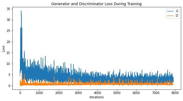
Losses versus training iterations
Below is a plot of the discriminator’s and generator’s losses versus training iterations.
%matplotlib inline

plt.figure(figsize=(10,5))
plt.title("Generator and Discriminator Loss During Training")
plt.plot(G_losses,label="G")
plt.plot(D_losses,label="D")
plt.xlabel("iterations")
plt.ylabel("Loss")
plt.legend()
<matplotlib.legend.Legend at 0x7f2ca90dd3d0>
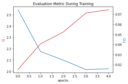
Evaluation Metric versus training iterations
Below is a plot of Evaluation versus training iterations.
As we can see IS increases sharply at first indicating the generator model is learning quickly how to generate faces. Unlike IS, FID is decreasing sharply at first similarly indicating the learning process of the generator model.
Note: Higher value of FID implies better results and lower value of IS implies better results.
fig, ax1 = plt.subplots()

plt.title("Evaluation Metric During Training")

color = 'tab:red'
ax1.set_xlabel('epochs')
ax1.set_ylabel('IS', color=color)
ax1.plot(is_values, color=color)

ax2 = ax1.twinx()

color = 'tab:blue'
ax2.set_ylabel('FID', color=color)
ax2.plot(fid_values, color=color)

fig.tight_layout()
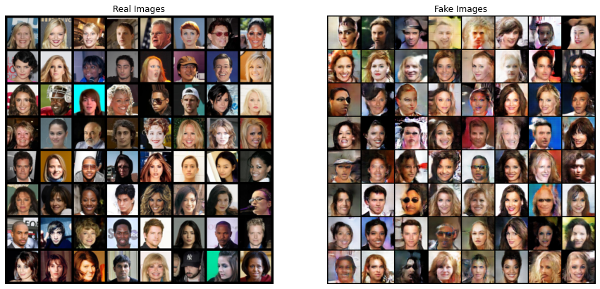
Real Images vs. Fake Images
Finally, lets take a look at some real images and fake images side by side.
%matplotlib inline

# Grab a batch of real images from the dataloader
real_batch = next(iter(train_dataloader))

# Plot the real images
plt.figure(figsize=(15,15))
plt.subplot(1,2,1)
plt.axis("off")
plt.title("Real Images")
plt.imshow(np.transpose(vutils.make_grid(real_batch[0][:64], padding=5, normalize=True).cpu(),(1,2,0)))

# Plot the fake images from the last epoch
plt.subplot(1,2,2)
plt.axis("off")
plt.title("Fake Images")
plt.imshow(np.transpose(vutils.make_grid(img_list[-1], padding=2, normalize=True).cpu(),(1,2,0)))
<matplotlib.image.AxesImage at 0x7f2b1b872250>